Program Memory: Method (part 1)

A neural network uses its weight to compute inputs and return outputs as computation results. Hence, the weight can be viewed as the neural network’s program. If we maintain a program memory of different weights responsible for various computation functions, we have a neural Universal Turing Machine. Obvious scenarios where a Program Memory may help:

• Multi-task learning
• A complicated task that can be decomposed into sub-tasks
• Continual learning
• Adaptive learning

Program Memory

A naïve approach treats each matrix weight of a neural network as a separate program and maintains the program memory as a 3d tensor. Formally, let $M_p\in R^{N\times w \times h}$ the program memory; we have $M_p(i)$ the $i$-th matrix weight $W\in R^{w \times h}$. $M_p$ can generally be just a list of weights of arbitrary sizes. However, we restrict $M_p$ to a tensor consisting of equal-size weights to compute fast with matrix multiplication.

Given the program memory, we need a mechanism to compose the program used in the neural network $\mathcal{N}$ to compute some input $x$. Assume we have this program (a.k.a working program) $W_p$, the computation runs as $y=\mathcal{N}(x;W_p)$. The network can have multiple weights or layers, so we actually need numerous working programs such that $y=\mathcal{N}(x;W_p^1,W_p^2,..,W_p^K)$ where $K$ is the number of weights required.

Now comes the core part of Program Memory: composing working program $W_p$. In computer programming, when we want to compute $x$, we call functions or programs that specialise in handling $x$. If we know $x$, we know $W_p$. Hence, the working program is also conditioned on the input $x$ as: $W_p=f(x;M_p)$. One simple way to compose the working program $W_p$ is using a linear combination of programs in $M_p$:

where the coefficients are generated by a neural network $w=g_\theta(x)$. This approach assumes that the network $g$ can learn to select the right program for $x$ without knowing the content of $M_p$. In the simple case of a single working program, it produces outputs:

Relation to Mixture of Experts. The above approach is closely related to a classic adaptive computing model named Mixture of Mixture of Experts (MoE;[1]). In MoE, the outputs of multiple neural networks (a.k.a programs) are linearly combined to compute $y$. Actually, they are equivalent when $\mathcal{N}$ is a single-layer neural network without any activation function. That is,

However, the fundamental difference is that MoE combines the outputs while Program Memory combines the programs. The outcome will be so different as $\mathcal{N}$ becomes non-linear and complicated.

Neural Stored-Program Memory

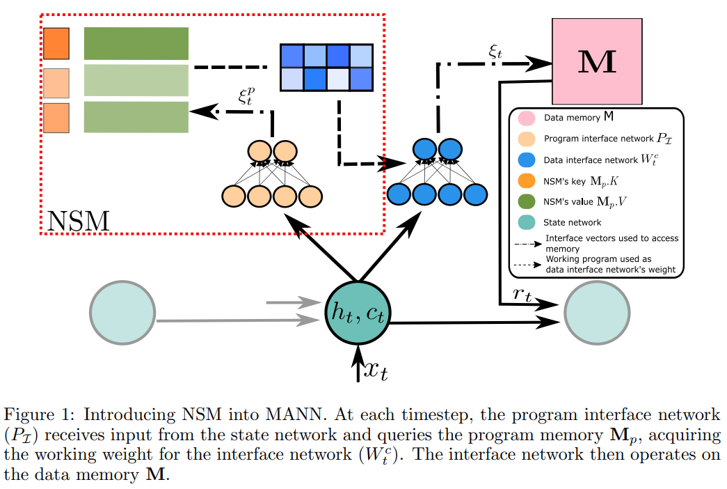
When a human programmer calls a function, it is unlikely that he doesn’t know anything about it. At least, he knows the purpose of the function, its name and where to find it. Neural Stored-Program Memory (NSM; [2]) realizes this idea by associating each program with an identifier (a.k.a a key in data structure or an address in computer architecture). The program memory now becomes a key-value memory: $M_p={M_p^k\in R^{N\times d},M_p^v\in R^{N\times w \times h}}$ . The key-value binding creates an indirection in the program/functional space. To work with the program (value), we can refer to its identifier (key). NSM accesses the program key by attention mechanism to generate the attention weight $w$ as follows,

where $q^p$ is the query and $\beta^p$ is the parameter controlling the sharpness of the softmax. They are generated by a neural network conditioned on $x$ :$q^p,\beta^p=g_\theta(x)$ . Given the weight $w$, NSM composes the working program in a similar manner as in Eq. (1):

Intuitively, if $w$ becomes a one-hot vector, we retrieve one of the $N$ programs in $M_p$ that can compute $x$. Most of the time, the working program will be a mixture of stored programs in $M_p$. This can be useful in a situation each program corresponds to some basic function, and we combine functions to compute complicated things (e.g. combining addition and multiplication programs to compute the expression $x=3\times5+6$).

Learning. There are two main components needed training. The first is the programs. Initialized randomly, the programs $M_p^v(i)$ and its keys $M_p^k(i)$ need training to work well with the data when they are accessed. The second is the routing network $g$ (also known as the program controller), which learns to select and combine relevant programs to produce working programs. By employing the attention mechanism, the whole system can be trained end-to-end using backpropagation.

In the original paper [2], the program memory is used to provide working weights for the controller of the Neural Turing Machine [3]. Hence, equipped with Program Memory, NTM becomes Neural Universal Turing Machine (NUTM, see Fig. 1).

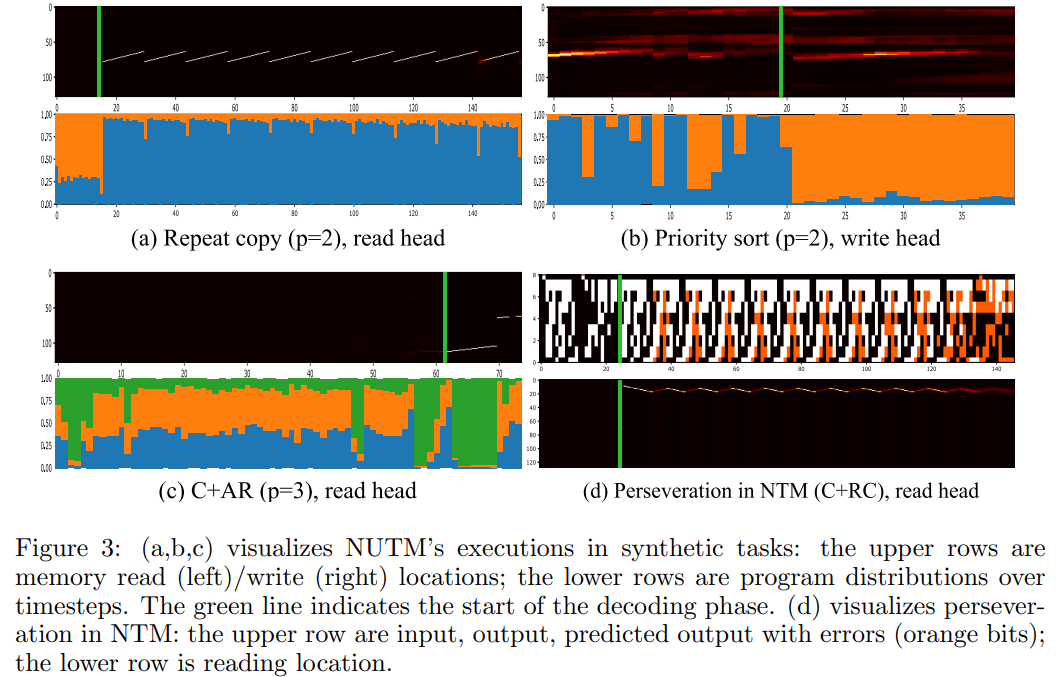
Adaptive Program Selection. As the attention weights are generated from the input $x$, we expect the program changes as $x$ changes. For example, in a sequence $x_{1,..,T}$ where a sub-sequence $x_{1,..t}$ should be handled by one program (e.g. store them into data memory) and the other $x_{t+1,T}$ handled by the other (e.g. sort them by values), we expect a big change in the attention pattern. As shown in Fig. 3, NUTM attends differently when the input sequence changes from encoding to decoding phase, leading to change in the controlling program and hence data addressing modes as expected.

Issues. Several prominent issues of Program Memory and the like are:

• Program collapse: there are multiple programs but only one or few are actually used. In other cases, the programs converge to the same weight. This will downgrade the capability of the universal neural network to a single-purpose model.

• Perseveration: the input changes, yet the program does not. This phenomenon can be attributed to a weak program controller which fails to respond to the change in the data.

• Overparameterization: the number of learnable parameters is redundant. As the current approaches treat a weight or a network as a program, the number of weights/networks scales as the program memory $M_p$ grows in size. The worst thing is that many parameters will be untouched and unshared, leading to inefficient learning and poor generalization. This can partially result in the program collapse. In the next article , we will consider a potential solution for this issue.

Reference

[1] Jacobs, R., Jordan, M. I., Nowlan. S. J. and Hinton, G. E. (1991) Adaptive mixtures of local experts. Neural Computation, 3, 79-87

[2] Le, Hung, Truyen Tran, and Svetha Venkatesh. “Neural Stored-program Memory.” In International Conference on Learning Representations. 2019.

[3] Graves, Alex, Greg Wayne, and Ivo Danihelka. “Neural turing machines.” arXiv preprint arXiv:1410.5401 (2014).